Introduction

This semestre’s course has come to an end. And in this course, I choose to do the project of cats and dogs. The goal of this project is to classify images of cats and dogs using the CNN architecture learned in course.

More specifically, given an image $X$, we have to use a trained CNN $f$ to calculate a prediction $y=f(x)$. This is a binary classification task, so the the label will be 0 for cat and 1 for dog.

Actually the images provided by kaggle can be quite difficult because there are backgrounds and other confusing visual part which will disturb and confuse the discriminative classification model’s classification ability. Also, some examples of cats and dogs’ faces look really similar, so we need to use a CNN to conduct feature learning and use the extracted feature to do classifications (typically by adding a MLP on top of last convolution-pooling layer). CNN is considered to be quite efficient to do image-based classification because it used local connections which dramatically reduced the number of parameters making the network easier to train, and it used weight sharing to extract many feature maps which will help better discimiate the image.

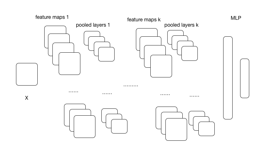
A typical CNN architecture is shown in Fig 1.

Experiments

Experiment 1.0

As a first try I used a 3 layered CNN, the configuration is a follows:

num_epochs= 100
image_shape = (128,128)
filter_sizes = [(5,5),(5,5),(5,5)]
feature_maps = [20,50,80]
pooling_sizes = [(2,2),(2,2),(2,2)]
mlp_hiddens = [1000]
output_size = 2
weights_init=Uniform(width=0.2)
step_rule=Scale(learning_rate=0.1)
Max_image_dim_limit_method = RandomFixedSizeCrop
Dataset_processing = rescale to 128*128

Here I used the RandomFixedSizeCrop to crop images into fixed 128*128 pixels, and using the Scale parameter update method (learning rule) from the blocks package. It will update the parameter in a step in the direction proportional to the previous step. And since it is used with GradientDescent alone, it willperform the steepest descent, which might not be a good choice.
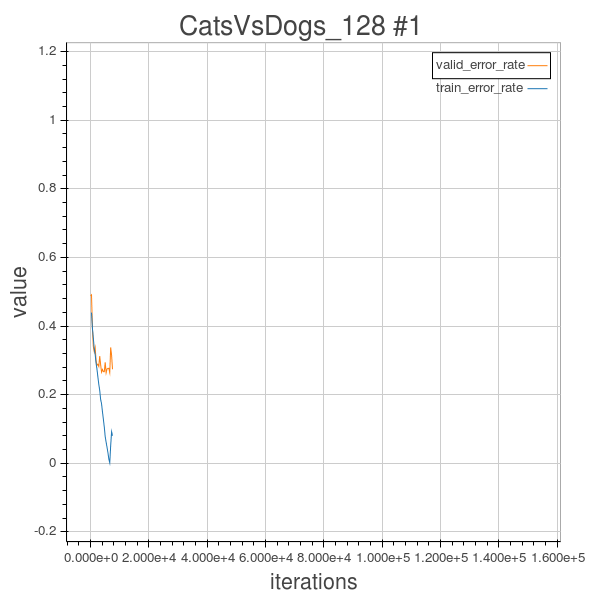
After 100 epochs, the training error = 26.31%, validation error = 25.77%

Experiment 1.1

A second try still with 3 convolutional layer network. A random fixed size crop doesn’t seems to be a good way to limit the size of image to a fixed size (e.g.128*128), so inspired by Florian’s blog, I used a modified version of MinImageDimension to do MaxImageDimension to limit the size of image to a fixed size. And also, I decreased the learning rate to 0.05 so the hyper parameter settings are as follows:

num_epochs= 100 early stopped
image_shape = (128,128)
filter_sizes = [(5,5),(5,5),(5,5)]
feature_maps = [20,50,80]
pooling_sizes = [(2,2),(2,2),(2,2)]
mlp_hiddens = [1000]
output_size = 2
weights_init=Uniform(width=0.2)
step_rule=Scale(learning_rate=0.05)
max_image_dim_limit_method= MaximumImageDimension
dataset_processing = rescale to 128*128

From the training curves, we can observe that the phenomenon of overfitting did occur, so I just stopped training at epoch 27 because the valid error no longer decreases. Next step, we will need to do something to regularize.

Experiment 1.2

In this experiment, before doing some regularization, I also changed the learning rule from the simple Scale method to Adam() which is implemented in Blocks package and is derived from Kingma et al. This will basically adaptively decay the learning rate as learning continues. And the other hyper parameters are unchanged from 1.1. But the overfitting still occurred. As shown in the training curve below. So we need to do something for regularization.

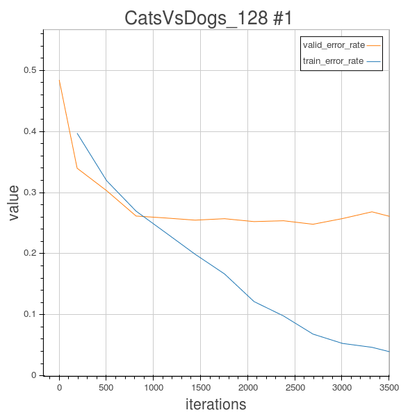
Experiment 1.3

As we can observe from the learning curve in experiment 1.2, after about 700 epochs, overfitting already occurred, the valid_error will stagnate at around 27%, and the training error will continues to decrease to about 5%, but that isn’t of any use…

So in order to overcome the overfitting phenomenon, there are a lot of methods to regularize, in this experiment 1.3, I uses the Random2DRotation Method to rotate each training image by a random degree, and keep their label untouched, so the model will learn different dogs or cats’images with different random rotated angles, and as we can see from the learning curve of experiment 1.3, this does help to reduce the overfitting. Globally, the training error and validation error curves are sticked together, and the validation error after 100 epochs is 19.4%.

The configurations are as follows:

num_epochs= 100 
image_shape = (128,128)
filter_sizes = [(5,5),(5,5),(5,5)]
feature_maps = [20,50,80]
pooling_sizes = [(2,2),(2,2),(2,2)]
mlp_hiddens = [1000]
output_size = 2
weights_init=Uniform(width=0.2)
step_rule=Adam()
max_image_dim_limit_method= MaximumImageDimension
dataset_processing = rescale to 128*128

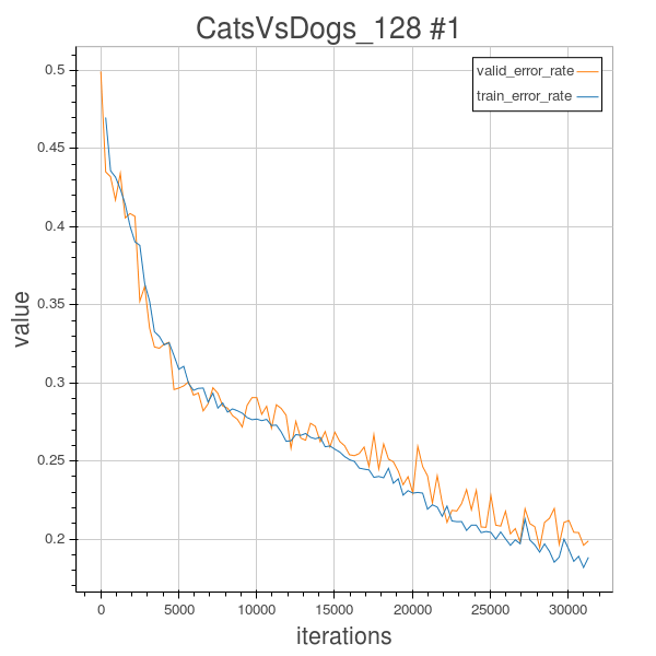
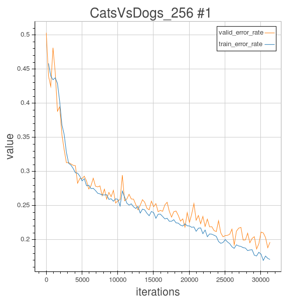
Experiment 2.01

In order to further extract more abstract feature to help classification, I tried some deeper achitectures in this experiment 2.01. I tried to use a 5 layered CNN, and the configuration is showed as below.

num_epochs= 100 
image_shape = (256,256)
filter_sizes = [(5,5),(5,5),(5,5),(5,5),(5,5)]
feature_maps = [20,40,60,80,100]
pooling_sizes = [(2,2),(2,2),(2,2),(2,2),(2,2)]
mlp_hiddens = [1000]
output_size = 2
weights_init=Uniform(width=0.2)
step_rule=Adam()
max_image_dim_limit_method= MaximumImageDimension
dataset_processing = rescale to 256*256

So in order to overcome the overfitting phenomenon, I still use the Random2DRotation Method to rotate each training image by a random degree, and keep their label untouched, so the model will learn different dogs or cats’images with different random rotated angles, and as we can see from the learning curve of experiment 2.01, this does help to reduce the overfitting. Globally, the training error and validation error curves are sticked together, and the validation error after 100 epochs is 19.6%.

Experiment 2.1

In this experiment 2.1 I tried to use a 6 layered CNN to conduct experiment, but I encountered the same strange thing as encountered by Florian. I used Adam() as update rule to do learning. During training the training error and validation error suddenly diverged and totally ruined the training process.

The configurations are as follows:

num_epochs= 120 
image_shape = (256,256)
filter_sizes = [(5,5),(5,5),(5,5),(5,5),(5,5),(5,5)]
feature_maps = [20,40,60,80,100, 120]
pooling_sizes = [(2,2),(2,2),(2,2)]
mlp_hiddens = [1000]
output_size = 2
weights_init=Uniform(width=0.2)
step_rule=Adam()
max_image_dim_limit_method= MaximumImageDimension
dataset_processing = rescale to 256*256

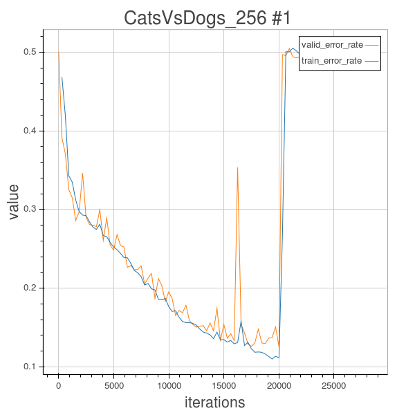
After some analysis, I learned that this might be caused by the initial setting of the learning rate. In the course we learned that if the learning rate is too small, the learning will be very slow, but if it is set too large, the learning will diverge.

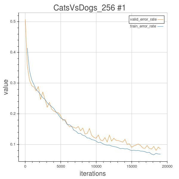
Experiment 2.2

In this experiment 2.2, I tried to reduce the filter sizes of the last 3 layers to (4,4), and still keep other configurations unchanged.

num_epochs= 61 
batch_size=64
image_shape = (256,256)
filter_sizes = [(5,5),(5,5),(5,5),(5,5),(5,5),(5,5)]
feature_maps = [20,40,60,80,100,120]
pooling_sizes = [(2,2),(2,2),(2,2),(2,2),(2,2),(2,2)]
mlp_hiddens = [1000]
output_size = 2
weights_init=Uniform(width=0.2)
step_rule=Adam(learning_rate=0.0005)
max_image_dim_limit_method= MaximumImageDimension
dataset_processing = rescale to 256*256

initial learning rate is very important, if it is set big, the optimization will oscillate, and if it is set too big, the optimization process will diverge, it is linked with the inverse of the biggest eigenvalue of the Hessian of the cost function. However if the learning rate is chosen to be too small, the learning will be very slow, and here, as we are using Adam() to decay the learning rate as time elapses, at the end stage the learning rate will be very small can the learning cannot go on effectively.

Also, the initial learning rate setting is important, because at the begining, we want to get down as fast as possible, so we cannot set too conservatively small learning rate. I’ve tried with trial and errors and concluded that 0.004 was too big, and the default 0.0002 is too small, this time I tried with 0.0005. It seemed work better!

Validation error=8.56% after 61 epochs

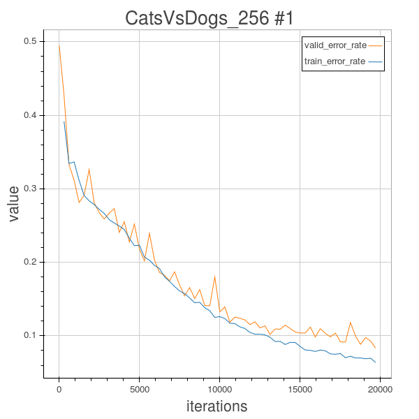
Experiment 2.3

As mentioned in last experiment 2.2, a learning rate of 0.0005 seems to work well for this 6 layered architecture. And in this experiment I added more feature maps and make the last convolutional layer havint 512 feature maps hoping this will help improve the discriminative power of the model.

num_epochs= 63 
batch_size=64
image_shape = (256,256)
filter_sizes = [(5,5),(5,5),(5,5),(5,5),(5,5),(5,5)]
feature_maps = [20,40,70,140,256, 512]
pooling_sizes = [(2,2),(2,2),(2,2),(2,2),(2,2),(2,2)]
mlp_hiddens = [1000]
output_size = 2
weights_init=Uniform(width=0.2)
step_rule=Adam(learning_rate=0.0005)
max_image_dim_limit_method= MaximumImageDimension
dataset_processing = rescale to 256*256

Training error = 3.33%, Validation error = 8.32% after 63 epochs.

Result, Discussion And Conclusion
Based on the validation error, the best model is the model 2.3 which has 6 convolutional layers with feature maps [20,40,70,140,256, 512]. its training error = 3.33%, validation error = 8.32% after uploading its predicted test label to Kaggle, its’s test error = 9.896%.

During this project, I have learned a lot. First, the theano and blocks package really provided an efficient way to quickly build some deep learning architecture. And I learned some basic usages of thoses tool although I’m still learning.

In this project, I tried several different hyper parameter settings, since training each network consumes a lot of time, due to time limitation, it’s limited to the experiments described above. And among those trial and errors, I’ved learned several things: 1. Deeper architecture does help to improve performance. If we compare the performance of 3 conv-layered CNN with the performance of 6 conv-layered CNN we can observe that the validation error for 3 layered CNN will be around 20%, while the validation error for 6 layered CNN will be around 10% if propered configured (the hyperparameters). This does make sense, since with deeper CNN, at each layer we typically add more feature maps, which will extract more higer level, more abstract features to help the model to improve its performance. 2. Regularization is very necessary. Actually we can observe that without random rotation of the training images, in those experiments, the training error will continue to go down whereas the validation error will stagnate around a higer value. In those cases overfitting occurs, i.e. the model will try to memeorize the training image and their corresponding training labels and fit the parameters to specifically fit those training images which will lead to bad generalization to unseen data. So by adding random image rotations to the training image, we can regularize. 3. Choice of (initial) learning rate is very important. From the experiment we can observe that a too small learning rate will result in very slow learning, however, a too big learning rate is not good either, it will make the gradient steps oscillate around the cost function surface and eventually diverge. From the course we learned that it is linked with the inverse of the biggest eigenvalue of the Hessian of the cost function. So a good choice of learning rate is important. For the 6 layered CNN in my experiment, after some trial and errors, I found that 0.0005 seems to work well as the initial learning rate for the Adam() optimization algorithm.

I have a learned a lot during this course project. But I’m still a starter in neural network models, and due to time and knowledge limitations, there are still many things to improve. In the future, it is worthwile to try other regularization techniques learned in course such as batch normalizations, and maybe other data augmentation schemes to do better regularization.